Case Study Enrichment Design
November 20, 2024
Case Study Enrichment Design
Population Enrichment Design
Closed Combination Test
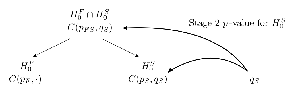
Combination tests to be performed for the closed system of hypotheses (\(G = 2\)) if subpopulation \(S\) referring to hypothesis \(H_0^S\) is selected for the second stage.
Population Enrichment Design
- Janssen training on June 2/9, 2022 and June 7/14, 2023
Vignette Enrichment Designs for Testing Rates with rpact available on www.rpact.com
Up to G = 4 populations in multi-stage designs with maximum of 6 stages (\(K \leq 6\)).
Can be applied to selection of one or more than one population.
The number of selected populations and the way of how to select populations needs not to be preplanned, different strategies can be specified.
Choice of combination test is free: inverse normal and Fisher combination test.
Data-driven recalculation of sample size is possible.
Choice of intersection tests is free. You can choose between Spiessens & Debois (\(G = 2\)), Bonferroni, Simes, and Sidak.
getSimulationEnrichment...(design =, effectList = , plannedSubjects = )
designThe trial design. If no trial design is specified, a fixed sample size design is used. In this case, Type I error ratealpha, Type II error ratebeta,twoSidedPower, andsidedcan be directly entered as argument where necessary.effectListList of subsets, prevalences, and effect sizes with columns and number of rows reflecting the different situations to consider (see examples).plannedSubjectsis a vector of lengthkMax(the number of stages of the design) that determines the number of cumulated (overall) subjects when the interim stages are planned. For two treatment arms, it is the number of subjects for both treatment arms. For multi-arm designs,plannedSubjectsrefers to the number of subjects per selected active arm.stratifiedAnalysisFor enrichment designs, typically a stratified analysis should be chosen. For testing rates, also a non-stratified analysis based on overall data can be performed. For survival data, only a stratified analysis is possible (see Brannath et al., 2009), default isTRUE.adaptationsA vector of lengthkMax - 1indicating whether or not an adaptation takes place at interim k, default isrep(TRUE, kMax - 1).typeOfSelectionThe way the treatment arms or populations are selected at interim. Five options are available:"best","rbest","epsilon","all", and"userDefined", default is"best".
For"rbest"(select therValuebest treatment arms/populations), the parameterrValuehas to be specified, for"epsilon"(select treatment arm/population not worse than epsilon compared to the best), the parameterepsilonValuehas to be specified. If"userDefined"is selected,"selectArmsFunction"or"selectPopulationsFunction"has to be specified.effectMeasureCriterion for treatment arm/population selection, either based on test statistic ("testStatistic") or effect estimate (difference for means and rates or hazard ratio for survival) ("effectEstimate"), default is"effectEstimate".successCriterionDefines when the study is stopped for efficacy at interim. Two options are available:"all"stops the trial if the efficacy criterion is fulfilled for all selected treatment arms/populations,"atLeastOne"stops if at least one of the selected treatment arms/populations is shown to be superior to control at interim, default is"all".epsilonValueFortypeOfSelection = "epsilon"(select treatment arm / population not worse than epsilon compared to the best), the parameterepsilonValuehas to be specified.rValueForypeOfSelection = "rbest"(select therValuebest treatment arms / populations), the parameterrValuehas to be specified.thresholdSelection criterion: treatment arm / population is selected only ifeffectMeasureexceedsthreshold, default is-Inf.thresholdcan also be a vector of lengthactiveArmsreferring to a separate threshold condition over the treatment arms.intersectionTestDefines the multiple test for the intersection hypotheses in the closed system of hypotheses. Four options are available in enrichment designs:"SpiessensDebois","Bonferroni","Simes", and"Sidak", default is"Simes".allocationRatioPlannedThe planned allocation ration1 / n2for a two treatment groups design, default is1. For multi-arm designs, it is the allocation ratio relating the active arm(s) to the control.minNumberOfSubjectsPerStageWhen performing a data driven sample size recalculation, the vectorminNumberOfSubjectsPerStagewith lengthkMaxdetermines the minimum number of subjects per stage (i.e., not cumulated), the first element is not taken into account. For two treatment arms, it is the number of subjects for both treatment arms. For multi-arm designsminNumberOfSubjectsPerStagerefers to the minimum number of subjects per selected active arm.maxNumberOfSubjectsPerStageWhen performing a data driven sample size recalculation, the vectormaxNumberOfSubjectsPerStagewith lengthkMaxdetermines the maximum number of subjects per stage (i.e., not cumulated), the first element is not taken into account. For two treatment arms, it is the number of subjects for both treatment arms. For multi-arm designsmaxNumberOfSubjectsPerStagerefers to the maximum number of subjects per selected active arm.conditionalPowerIfconditionalPowertogether withminNumberOfSubjectsPerStageandmaxNumberOfSubjectsPerStage(orminNumberOfEventsPerStageandmaxNumberOfEventsPerStagefor survival designs) is specified, a sample size recalculation based on the specified conditional power is performed. It is defined as the power for the subsequent stage given the current data. By default, the conditional power will be calculated under the observed effect size. Optionally, you can also specifythetaH1andstDevH1(for simulating means),pi1H1andpi2H1(for simulating rates), orthetaH1(for simulating hazard ratios) as parameters under which it is calculated and the sample size recalculation is performed.thetaH1If specified, the value of the alternative under which the conditional power or sample size recalculation calculation is performed.stDevH1If specified, the value of the standard deviation under which the conditional power or sample size recalculation calculation is performed, default is the value ofstDev.maxNumberOfIterationsThe number of simulation iterations, default is1000.seedThe seed to reproduce the simulation, default is a random seed.calcSubjectsFunctionOptionally, a function can be entered that defines the way of performing the sample size recalculation. By default, sample size recalculation is performed with conditional power with specifiedminNumberOfSubjectsPerStageandmaxNumberOfSubjectsPerStage(see details and examples).
New
selectPopulationsFunctionOptionally, a function can be entered that defines the way of how populations are selected. This function is allowed to depend oneffectVectorwith lengthpopulations,stage,conditionalPower,conditionalCriticalValue,plannedSubjects/plannedEvents,allocationRatioPlanned,selectedPopulations,thetaH1(for means and survival),stDevH1(for means),overallEffects, and for rates additionally:piTreatmentsH1,piControlH1,overallRates, andoverallRatesControl. (see examples).
showStatisticsIfTRUE, summary statistics of the simulated data are displayed for theprintcommand, otherwise the output is suppressed, default isFALSE.
Example Enrichment Simulation Means
Example G = 2: Assess a population selection strategy with one subset population
If the subset is better than the full population, then the subset is selected for the second stage, otherwise the full. Print and plot design characteristics.
library(rpact)
# Define design
ds <- getDesignInverseNormal(
    kMax = 2,
    typeOfDesign = "noEarlyEfficacy"
)
# Define subgroups and their prevalences
subGroups <- c("S", "R") # fixed names!
prevalences <- c(0.2, 0.8)
# Define effect matrix and variability
effectR <- 0.2
m <- c()
for (effectS in seq(0, 0.5, 0.25)) {
    m <- c(m, effectS, effectR)
}
# Define effect list
effects <- matrix(m, byrow = TRUE, ncol = 2)
stDev <- c(0.4, 0.8)
el <- list(subGroups=subGroups, prevalences=prevalences,
            stDevs = stDev, effects = effects)
# Perform simulation
simResultsPE <- getSimulationEnrichmentMeans(
    design = ds,
    effectList = el,
    typeOfSelection = "best",
    intersectionTest = "SpiessensDebois",
    plannedSubjects = c(50, 100),
    maxNumberOfIterations = 100)
simResultsPE |> print()
Simulation of enrichment means (inverse normal combination test design):
Design parameters:
Information rates : 0.500, 1.000
Critical values : Inf, 1.960
Futility bounds (non-binding) : -Inf
Cumulative alpha spending : 0.0000, 0.0250
Local one-sided significance levels : 0.0000, 0.0250
Significance level : 0.0250
Test : one-sided
User defined parameters:
Maximum number of iterations : 100
Planned cumulative subjects : 50, 100
Effect list [Sub-groups] : S, R
Effect list [Prevalences] : 0.2, 0.8
Effect list [Standard deviations] : 0.4, 0.8
Effect list [Effects] (1) : 0, 0.2
Effect list [Effects] (2) : 0.25, 0.2
Effect list [Effects] (3) : 0.5, 0.2
Intersection test : SpiessensDebois
Derived from user defined parameters:
Populations : 2
Default parameters:
Seed : -1311651743
Planned allocation ratio : 1
Calculate subjects function : default
Stratified analysis : TRUE
Adaptations : TRUE
Type of selection : best
Effect measure : effectEstimate
Success criterion : all
Epsilon value : NA
r value : NA
Threshold : -Inf
Results:
Iterations [1] : 100, 100, 100
Iterations [2] : 100, 100, 100
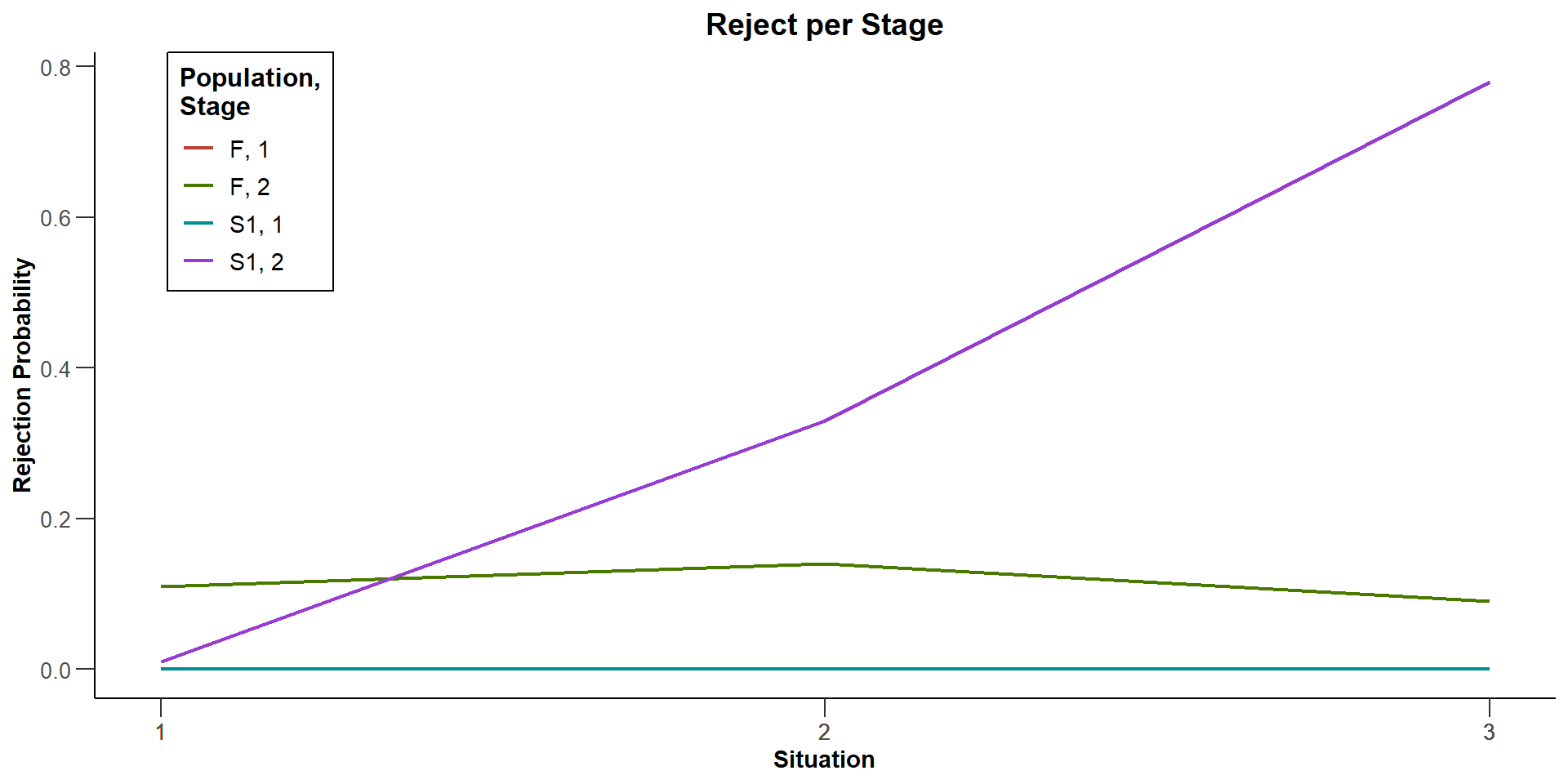
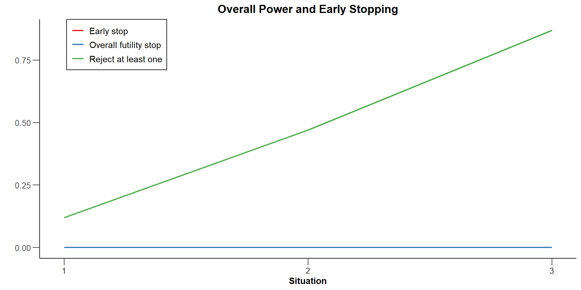
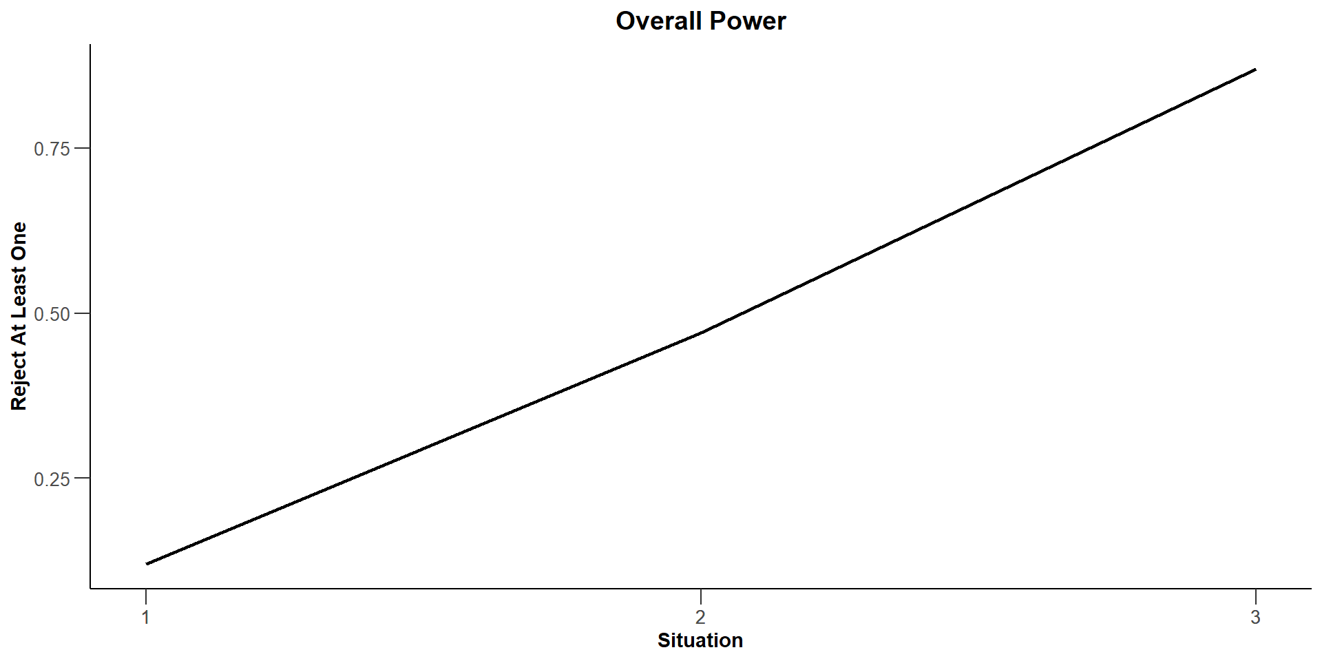
Reject at least one : 0.1200, 0.4700, 0.8700
Rejected populations per stage (S) [1] : 0, 0, 0
Rejected populations per stage (S) [2] : 0.01, 0.33, 0.78
Rejected populations per stage (F) [1] : 0, 0, 0
Rejected populations per stage (F) [2] : 0.11, 0.14, 0.09
Futility stop per stage : 0.0000, 0.0000, 0.0000
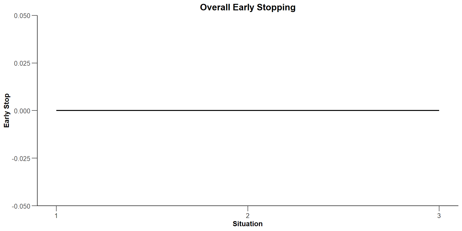
Early stop : 0.0000, 0.0000, 0.0000
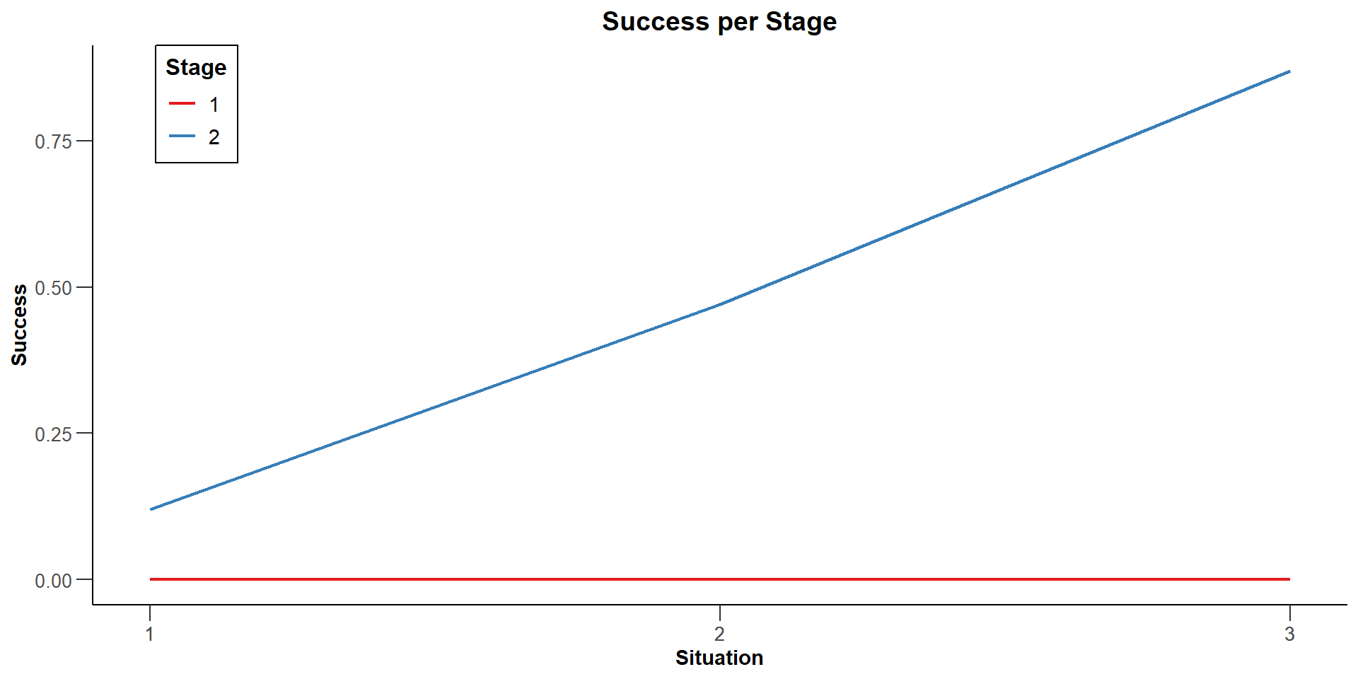
Success per stage [1] : 0.0000, 0.0000, 0.0000
Success per stage [2] : 0.1200, 0.4700, 0.8700
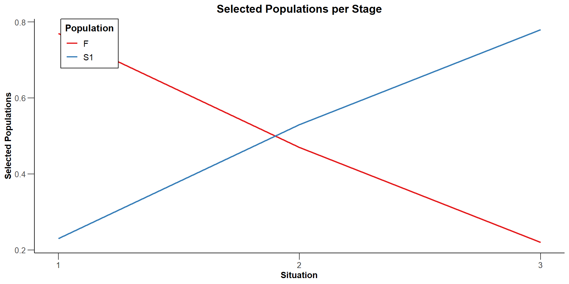
Selected populations (S) [1] : 1, 1, 1
Selected populations (S) [2] : 0.23, 0.53, 0.78
Selected populations (F) [1] : 1, 1, 1
Selected populations (F) [2] : 0.77, 0.47, 0.22
Number of populations [1] : 2, 2, 2
Number of populations [2] : 1, 1, 1
Expected number of subjects : 100, 100, 100
Sample sizes (S) [1] : 10, 10, 10
Sample sizes (S) [2] : 19.2, 31.2, 41.2
Sample sizes (R) [1] : 40, 40, 40
Sample sizes (R) [2] : 30.8, 18.8, 8.8
Conditional power (achieved) [1] : NA, NA, NA
Conditional power (achieved) [2] : 0.0885, 0.2704, 0.5295
Legend:
(i): results of situation i
[k]: values at stage k
S[i]: population i
F: full population
R: remaining populationExample Enrichment Simulation Means
Example G = 2: Assess a population selection strategy with one subset population
Simulation of a continuous endpoint (enrichment design)
Sequential analysis with a maximum of 2 looks (inverse normal combination test design), one-sided overall significance level 2.5%. The results were simulated for a population enrichment comparisons for means (treatment vs. control, 2 populations), H0: mu(treatment) - mu(control) = 0, power directed towards larger values, H1: effect as specified, subgroups = c(S, R), prevalences = c(0.2, 0.8), standard deviations = c(0.4, 0.8), planned cumulative sample size = c(50, 100), intersection test = SpiessensDebois, selection = best, effect measure based on effect estimate, success criterion: all, simulation runs = 100, seed = -1311651743.
| Stage | 1 | 2 |
|---|---|---|
| Fixed weight | 0.707 | 0.707 |
| Cumulative alpha spent | 0 | 0.0250 |
| Stage levels (one-sided) | 0 | 0.0250 |
| Efficacy boundary (z-value scale) | Inf | 1.960 |
| Reject at least one, effects = c(0, 0.2) | 0.1200 | |
| Reject at least one, effects = c(0.25, 0.2) | 0.4700 | |
| Reject at least one, effects = c(0.5, 0.2) | 0.8700 | |
| Rejected populations per stage, effects = c(0, 0.2) | ||
| Subset S | 0 | 0.0100 |
| Full population F | 0 | 0.1100 |
| Rejected populations per stage, effects = c(0.25, 0.2) | ||
| Subset S | 0 | 0.3300 |
| Full population F | 0 | 0.1400 |
| Rejected populations per stage, effects = c(0.5, 0.2) | ||
| Subset S | 0 | 0.7800 |
| Full population F | 0 | 0.0900 |
| Success per stage, effects = c(0, 0.2) | 0 | 0.1200 |
| Success per stage, effects = c(0.25, 0.2) | 0 | 0.4700 |
| Success per stage, effects = c(0.5, 0.2) | 0 | 0.8700 |
| Stage-wise number of subjects, effects = c(0, 0.2) | ||
| Subset S | 10.0 | 19.2 |
| Remaining population R | 40.0 | 30.8 |
| Stage-wise number of subjects, effects = c(0.25, 0.2) | ||
| Subset S | 10.0 | 31.2 |
| Remaining population R | 40.0 | 18.8 |
| Stage-wise number of subjects, effects = c(0.5, 0.2) | ||
| Subset S | 10.0 | 41.2 |
| Remaining population R | 40.0 | 8.8 |
| Expected number of subjects under H1, effects = c(0, 0.2) | 100.0 | |
| Expected number of subjects under H1, effects = c(0.25, 0.2) | 100.0 | |
| Expected number of subjects under H1, effects = c(0.5, 0.2) | 100.0 | |
| Overall exit probability, effects = c(0, 0.2) | 0 | |
| Overall exit probability, effects = c(0.25, 0.2) | 0 | |
| Overall exit probability, effects = c(0.5, 0.2) | 0 | |
| Selected populations, effects = c(0, 0.2) | ||
| Subset S | 1.0000 | 0.2300 |
| Full population F | 1.0000 | 0.7700 |
| Selected populations, effects = c(0.25, 0.2) | ||
| Subset S | 1.0000 | 0.5300 |
| Full population F | 1.0000 | 0.4700 |
| Selected populations, effects = c(0.5, 0.2) | ||
| Subset S | 1.0000 | 0.7800 |
| Full population F | 1.0000 | 0.2200 |
| Number of populations, effects = c(0, 0.2) | 2.000 | 1.000 |
| Number of populations, effects = c(0.25, 0.2) | 2.000 | 1.000 |
| Number of populations, effects = c(0.5, 0.2) | 2.000 | 1.000 |
| Conditional power (achieved), effects = c(0, 0.2) | 0.0885 | |
| Conditional power (achieved), effects = c(0.25, 0.2) | 0.2704 | |
| Conditional power (achieved), effects = c(0.5, 0.2) | 0.5295 | |
| Exit probability for efficacy | 0 |


Example Enrichment Simulation Means
Example G = 3: Assess the design characteristics of a user defined selection strategy
Three-stage design with no interim efficacy stop using the inverse normal method for combining the stages. Only the second interim is used for a selecting of a study population.
# Define design
ds <- getDesignInverseNormal(
    kMax = 3,
    typeOfDesign = "noEarlyEfficacy"
)

# Define selection function
mySelection <- function(effectVector, stage) {
    selectedPopulations <- rep(TRUE, 3)
    if (stage == 2) {
        selectedPopulations <- (effectVector >= c(1, 2, 3))
    }
    return(selectedPopulations)
}
# Define subgroups and their prevalences
subGroups <- c("S1", "S12", "S2", "R") # fixed names!
prevalences <- c(0.2, 0.3, 0.4, 0.1)
effectR <- 1.5
effectS12 <- 5
m <- c()
for (effectS1 in seq(0, 5, 5)) {
for (effectS2 in seq(0, 5, 5)) {
m <- c(m, effectS1, effectS12, effectS2, effectR)
}
}
effects <- matrix(m, byrow = TRUE, ncol = 4)
stDev <- 10Example Enrichment Simulation Means
Example G = 3: Assess the design characteristics of a user defined selection strategy
# Define effect list
el <- list(subGroups=subGroups, prevalences=prevalences,
     stDevs = stDev, effects = effects
)

# Perform simulation
simResultsPE <- getSimulationEnrichmentMeans(
    design = ds,
    effectList = el,
    typeOfSelection = "userDefined",
    selectPopulationsFunction = mySelection,
    intersectionTest = "Simes",
    plannedSubjects = c(50, 100, 150),
    maxNumberOfIterations = 100
)
simResultsPE |> print()
Simulation of enrichment means (inverse normal combination test design):
Design parameters:
Information rates : 0.333, 0.667, 1.000
Critical values : Inf, Inf, 1.960
Futility bounds (non-binding) : -Inf, -Inf
Cumulative alpha spending : 0.0000, 0.0000, 0.0250
Local one-sided significance levels : 0.0000, 0.0000, 0.0250
Significance level : 0.0250
Test : one-sided
User defined parameters:
Maximum number of iterations : 100
Planned cumulative subjects : 50, 100, 150
Effect list [Sub-groups] : S1, S2, S12, R
Effect list [Prevalences] : 0.2, 0.4, 0.3, 0.1
Effect list [Standard deviations] : 10, 10, 10, 10
Effect list [Effects] (1) : 0, 0, 5, 1.5
Effect list [Effects] (2) : 0, 5, 5, 1.5
Effect list [Effects] (3) : 5, 0, 5, 1.5
Effect list [Effects] (4) : 5, 5, 5, 1.5
Type of selection : userDefined
Derived from user defined parameters:
Populations : 3
Default parameters:
Seed : -1784099048
Planned allocation ratio : 1
Calculate subjects function : default
Intersection test : Simes
Stratified analysis : TRUE
Adaptations : TRUE, TRUE
Effect measure : effectEstimate
Success criterion : all
Results:
Iterations [1] : 100, 100, 100, 100
Iterations [2] : 100, 100, 100, 100
Iterations [3] : 81, 94, 90, 98
Reject at least one : 0.1800, 0.5400, 0.4600, 0.7400
Rejected populations per stage (S1) [1] : 0, 0, 0, 0
Rejected populations per stage (S1) [2] : 0, 0, 0, 0
Rejected populations per stage (S1) [3] : 0.14, 0.3, 0.46, 0.56
Rejected populations per stage (S2) [1] : 0, 0, 0, 0
Rejected populations per stage (S2) [2] : 0, 0, 0, 0
Rejected populations per stage (S2) [3] : 0.13, 0.54, 0.14, 0.64
Rejected populations per stage (F) [1] : 0, 0, 0, 0
Rejected populations per stage (F) [2] : 0, 0, 0, 0
Rejected populations per stage (F) [3] : 0.07, 0.43, 0.22, 0.65
Overall futility stop : 0.1900, 0.0600, 0.1000, 0.0200
Futility stop per stage [1] : 0.0000, 0.0000, 0.0000, 0.0000
Futility stop per stage [2] : 0.1900, 0.0600, 0.1000, 0.0200
Early stop [1] : 0.0000, 0.0000, 0.0000, 0.0000
Early stop [2] : 0.1900, 0.0600, 0.1000, 0.0200
Success per stage [1] : 0.0000, 0.0000, 0.0000, 0.0000
Success per stage [2] : 0.0000, 0.0000, 0.0000, 0.0000
Success per stage [3] : 0.1200, 0.3300, 0.2800, 0.5000
Selected populations (S1) [1] : 1, 1, 1, 1
Selected populations (S1) [2] : 1, 1, 1, 1
Selected populations (S1) [3] : 0.75, 0.83, 0.89, 0.94
Selected populations (S2) [1] : 1, 1, 1, 1
Selected populations (S2) [2] : 1, 1, 1, 1
Selected populations (S2) [3] : 0.51, 0.91, 0.51, 0.93
Selected populations (F) [1] : 1, 1, 1, 1
Selected populations (F) [2] : 1, 1, 1, 1
Selected populations (F) [3] : 0.22, 0.73, 0.4, 0.85
Number of populations [1] : 3, 3, 3, 3
Number of populations [2] : 3, 3, 3, 3
Number of populations [3] : 1.827, 2.628, 2, 2.776
Expected number of subjects : 140.5, 147, 145, 149
Sample sizes (S1 only) [1] : 10, 10, 10, 10
Sample sizes (S1 only) [2] : 10, 10, 10, 10
Sample sizes (S1 only) [3] : 13.3, 9.7, 14, 10.3
Sample sizes (S2 only) [1] : 20, 20, 20, 20
Sample sizes (S2 only) [2] : 20, 20, 20, 20
Sample sizes (S2 only) [3] : 13.9, 20.3, 12.4, 19.5
Sample sizes (S12) [1] : 15, 15, 15, 15
Sample sizes (S12) [2] : 15, 15, 15, 15
Sample sizes (S12) [3] : 21.5, 16.2, 21.3, 15.9
Sample sizes (R) [1] : 5, 5, 5, 5
Sample sizes (R) [2] : 5, 5, 5, 5
Sample sizes (R) [3] : 1.4, 3.9, 2.2, 4.3
Conditional power (achieved) [1] : NA, NA, NA, NA
Conditional power (achieved) [2] : 0, 0, 0, 0
Conditional power (achieved) [3] : 0.2298, 0.5244, 0.3347, 0.6631
Legend:
(i): results of situation i
[k]: values at stage k
S[i]: population i
F: full population
R: remaining population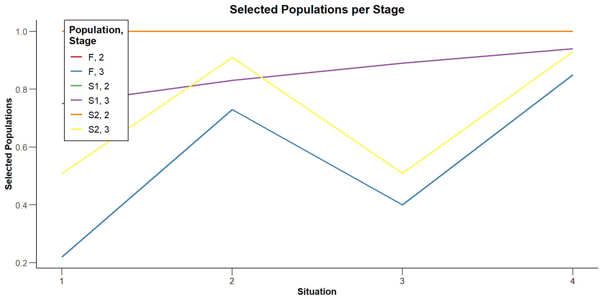
Simulation Enrichment Rates
getSimulationEnrichmentRates(effectList = , plannedSubjects = )
…
stratifiedAnalysisFor enrichment designs, typically a stratified analysis should be chosen. For testing rates, also a non-stratified analysis based on overall data can be performed. For survival data, only a stratified analysis is possible (see Brannath et al., 2009), default isTRUE.directionUpperSpecifies the direction of the alternative, only applicable for one-sided testing; default isTRUEwhich means that larger values of the test statistics yield smaller p-values.effectListList of effect sizes with columns and number of rows reflecting the different situations to consider (see examples).
Simulation Enrichment Rates
Example G = 2
# Define effect list
subGroups <- c("S", "R")
prevalences <- c(0.4, 0.6)
piControl <- c(0.3, 0.4)
range1 <- piControl[1] + seq(0.0, 0.2, 0.1)
range2 <- piControl[2] + seq(0.0, 0.2, 0.1)
piTreatments <- c()
for (x1 in range1) {
    for (x2 in range2) {
        piTreatments <- c(piTreatments, x1, x2)
    }
}
effectList <- list(
    subGroups = subGroups,
    prevalences = prevalences,
    piControl = piControl,
    piTreatments = matrix(piTreatments, byrow = TRUE, ncol = 2))
effectList
$subGroups
[1] "S" "R"
$prevalences
[1] 0.4 0.6
$piControl
[1] 0.3 0.4
$piTreatments
[,1] [,2]
[1,] 0.3 0.4
[2,] 0.3 0.5
[3,] 0.3 0.6
[4,] 0.4 0.4
[5,] 0.4 0.5
[6,] 0.4 0.6
[7,] 0.5 0.4
[8,] 0.5 0.5
[9,] 0.5 0.6Simulation Enrichment Survival
getSimulationEnrichmentSurvival(effectList = , plannedEvents = )
…
plannedEventsis a vector of lengthkMax(the number of stages of the design) that determines the number of cumulated (overall) events in survival designs when the interim stages are planned. For two treatment arms, it is the number of events for both treatment arms. For multi-arm designs,plannedEventsrefers to the overall number of events for the selected arms plus control.directionUpperSpecifies the direction of the alternative, only applicable for one-sided testing; default isTRUEwhich means that larger values of the test statistics yield smaller p-values.effectListList of effect sizes with columns and number of rows reflecting the different situations to consider (see examples).
Simulation Enrichment Survival
Example G = 2: Effect list defined through event rates yielding a range of hazard ratios in the subsets.
# Define effect list
subGroups <- c("S", "R")
prevalences <- c(0.40, 0.60)
piControl <- c(0.3, 0.4)
effectRangeS <- seq(0, 0.2, 0.05)
effectRangeR <- rep(0.05, length(effectRangeS))
hazardRatios <- matrix(c(
    log(1 - piControl[1] + effectRangeS) /
        log(1 - piControl[1]),
    log(1 - piControl[2] + effectRangeR) /
        log(1 - piControl[2])),
    byrow = FALSE, ncol = 2
)
effectList <- list(
    subGroups = subGroups,
    prevalences = prevalences,
    hazardRatios = hazardRatios
)

effectList
$subGroups
[1] "S" "R"
$prevalences
[1] 0.4 0.6
$hazardRatios
[,1] [,2]
[1,] 1.0000000 0.8433072
[2,] 0.8065665 0.8433072
[3,] 0.6256216 0.8433072
[4,] 0.4556500 0.8433072
[5,] 0.2953965 0.8433072Background of Simulation
- For simulating means, we create normally distributed test statistics with expectation according to the effect and the information in the subset.
- For simulating rates, we create random number of events according to assumed probabilities and the information in the subset.
- Information per subset clear for simulating means and simulating rates: sample sizes multiplied with prevalences of the subsets.
- Simulating log-rank statistics: information according to estimated number of events in the subsets \(1,\ldots,M\) as follows:
Simulation Enrichment Survival
- Given the cumulated events over the stages, \(d_1,\ldots,d_K\), the specified hazard ratios \(\omega_1,\ldots,\omega_M\) in the subsets and planned allocation ratio \(r\), at the first stage (\(k = 1\)) the events to be observed in the subset \(m\) with given prevalence \(\upsilon_m\) of the subsets are estimated through \[ d_1^m = \frac{(r\!\cdot\!\omega_m + 1)\!\cdot\!\upsilon_m}{\sum_{\tilde m = 1}^M (r\!\cdot\!\omega_{\tilde m} + 1)\!\cdot\!\upsilon_{\tilde m}} \cdot d_1 \;,\;m = 1,\ldots,M. \]
- From that, the normally distributed log-rank statistics \[ \text{LR}_m^* \sim N\big(\sqrt{d_1^m}\cdot \frac{\sqrt{r}}{1+r} \cdot \log(\omega_m), 1\big), m = 1,\ldots, M, \] are generated and, for sub-population \(S_g\), \[ \text{LR}_g^* = \sum\nolimits_{m \in S_g} \sqrt{d_1^m} \cdot \text{LR}_m^* / \sqrt{\sum\nolimits_{m \in S_g} d_1^m}, g = 1,\ldots, G, \] is calculated, where the summation runs over the indices of subsets \(m\) belonging to the sub-population \(S_g\).
Simulation Enrichment Survival
For the next stages, the log-rank statistics are generated analogously taking into account the adjusted prevalences \[\tilde{\upsilon}_m = \frac{\upsilon_m}{\sum_{{\tilde m} \in {\cal M}_k}\upsilon_{\tilde m}}\] of the selected subsets, where \({\cal M}_k\) denotes the set of selected subsets for stage \(k\) (all other prevalences are set equal to \(0\)).
This way of generating normally distributed log-rank statistics approximates the simulation of stratified log-rank statistics with specified hazard ratios and prevalences in the subsets (under the assumed assumptions).
Approximation may perform badly if the control hazards in the considered subsets cannot assumed to be constant.
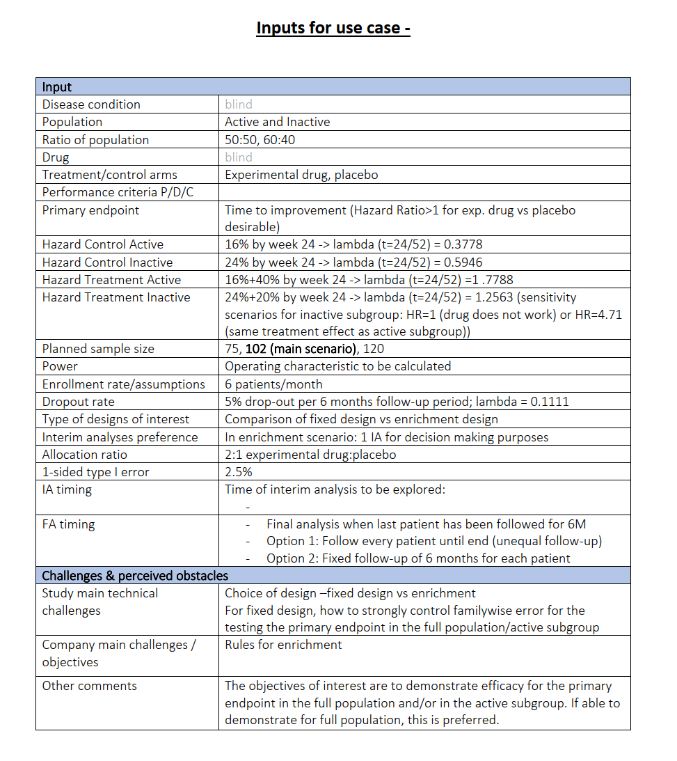
Case Study Enrichment Design
Parameters
One subset S (“active”), one remainder R (“inactive”)
Treatment arms experimental T vs. placebo C
Prevalence of S is 50% or 60%
Endpoint time to improvement \(H_1: \omega = \frac{\lambda_T}{\lambda_C} > 1\)
Effect sizes
S:
\(\lambda_T\) = -log(1 - 0.56) / (24 / 52) = 1.7788
\(\lambda_C\) = -log(1 - 0.16) / (24 / 52) = 0.3778
\(\qquad\omega = 4.709\)R:
\(\lambda_T\) = -log(1 - 0.44) / (24 / 52) = 1.2563
\(\lambda_C\) = -log(1 - 0.24) / (24 / 52) = 0.5946
\(\qquad\omega = 2.113\)
Event driven trial
Sample size
Sample size calculation for a survival endpoint
Fixed sample analysis, one-sided significance level 2.5%, power 80%. The results were calculated for a two-sample logrank test, H0: hazard ratio = 1, H1: hazard ratio as specified, control pi(2) = 0.2, event time = 12, accrual time = 12, follow-up time = 6.
| Stage | Fixed |
|---|---|
| Stage level (one-sided) | 0.0250 |
| Efficacy boundary (z-value scale) | 1.960 |
| Efficacy boundary (t), HR = 4.709 | 2.956 |
| Efficacy boundary (t), HR = 2.113 | 1.688 |
| Number of subjects, HR = 4.709 | 31.4 |
| Number of subjects, HR = 2.113 | 197.4 |
| Number of events, HR = 4.709 | 13.1 |
| Number of events, HR = 2.113 | 56.1 |
| Analysis time | 18.00 |
| Expected study duration under H1, HR = 4.709 | 18.00 |
| Expected study duration under H1, HR = 2.113 | 18.00 |
Legend:
- (t): treatment effect scale
- HR: hazard ratio
Active Population S
getSampleSizeSurvival(
    pi1 = 0.56,
    pi2 = 0.16,
    eventTime = 24 / 4,
    maxNumberOfSubjects = 102,
    accrualIntensity = 6
) |> summary()
Sample size calculation for a survival endpoint
Fixed sample analysis, one-sided significance level 2.5%, power 80%. The results were calculated for a two-sample logrank test, H0: hazard ratio = 1, H1: treatment pi(1) = 0.56, control pi(2) = 0.16, number of subjects = 102, event time = 6, accrual time = 17, accrual intensity = 6.
| Stage | Fixed |
|---|---|
| Stage level (one-sided) | 0.0250 |
| Efficacy boundary (z-value scale) | 1.960 |
| Efficacy boundary (t) | 2.956 |
| Number of subjects | 102.0 |
| Number of events | 13.1 |
| Analysis time | 8.41 |
| Expected study duration under H1 | 8.41 |
Legend:
- (t): treatment effect scale
Inactive Population R
getSampleSizeSurvival(
    pi1 = 0.44,
    pi2 = 0.24,
    eventTime = 24 / 4,
    maxNumberOfSubjects = 102,
    accrualIntensity = 6
) |> summary()
Sample size calculation for a survival endpoint
Fixed sample analysis, one-sided significance level 2.5%, power 80%. The results were calculated for a two-sample logrank test, H0: hazard ratio = 1, H1: treatment pi(1) = 0.44, control pi(2) = 0.24, number of subjects = 102, event time = 6, accrual time = 17, accrual intensity = 6.
| Stage | Fixed |
|---|---|
| Stage level (one-sided) | 0.0250 |
| Efficacy boundary (z-value scale) | 1.960 |
| Efficacy boundary (t) | 1.688 |
| Number of subjects | 102.0 |
| Number of events | 56.1 |
| Analysis time | 21.22 |
| Expected study duration under H1 | 21.22 |
Legend:
- (t): treatment effect scale
Expected Number of Events for 50% prevalence
getSampleSizeSurvival(
    pi1 = (0.44 + 0.56)/2,
    pi2 = (0.24 + 0.16)/2,
    eventTime = 24 / 4,
    maxNumberOfSubjects = 102,
    accrualIntensity = 6
) |> fetch(eventsFixed)
eventsFixed
24.43884
First attempt
Plan the trial with 12 events at interim
Enrichment Design with One Interim Stage
ds <- getDesignInverseNormal(
  alpha = 0.025,
  informationRates = c(0.5, 1),
  typeOfDesign = "noEarlyEfficacy"
)
# Define effect list
subGroups <- c("S", "R")
prevalences <- c(0.50, 0.50)
piControl <- c(0.16, 0.24)
effectRangeS <- seq(0, 0.4, 0.1)
effectRangeR <- rep(0.20, length(effectRangeS))
hazardRatios <- matrix(c(
    log(1 - (piControl[1] + effectRangeS)) /
        log(1 - piControl[1]),
    log(1 - (piControl[2] + effectRangeR)) /
        log(1 - piControl[2])),
    byrow = FALSE, ncol = 2
)
el <- list(
    subGroups = subGroups,
    prevalences = prevalences,
    hazardRatios = hazardRatios
)
el
$subGroups
[1] "S" "R"
$prevalences
[1] 0.5 0.5
$hazardRatios
[,1] [,2]
[1,] 1.000000 2.112757
[2,] 1.726982 2.112757
[3,] 2.559670 2.112757
[4,] 3.534122 2.112757
[5,] 4.708716 2.112757Enrichment Design with One Interim Stage:
“select all”
simEnrichment1 <- getSimulationEnrichmentSurvival(
    design = ds,
    effectList = el,
    typeOfSelection = "all",
    intersectionTest = "Simes",
    plannedEvents = c(12, 24),
    maxNumberOfIterations = 2000
)
simEnrichment1 |> summary()
Simulation of a survival endpoint (enrichment design)
Sequential analysis with a maximum of 2 looks (inverse normal combination test design), one-sided overall significance level 2.5%. The results were simulated for a population enrichment logrank test (treatment vs. control, 2 populations), H0: hazard ratio = 1, power directed towards larger values, H1: hazard ratios as specified, subgroups = c(S, R), prevalences = c(0.5, 0.5), planned cumulative events = c(12, 24), intersection test = Simes, selection = all, effect measure based on effect estimate, success criterion: all, simulation runs = 2000, seed = 2010574830.
| Stage | 1 | 2 |
|---|---|---|
| Fixed weight | 0.707 | 0.707 |
| Cumulative alpha spent | 0 | 0.0250 |
| Stage levels (one-sided) | 0 | 0.0250 |
| Efficacy boundary (z-value scale) | Inf | 1.960 |
| Reject at least one, hazard ratios = c(1, 2.113) | 0.1160 | |
| Reject at least one, hazard ratios = c(1.727, 2.113) | 0.2560 | |
| Reject at least one, hazard ratios = c(2.56, 2.113) | 0.4655 | |
| Reject at least one, hazard ratios = c(3.534, 2.113) | 0.7030 | |
| Reject at least one, hazard ratios = c(4.709, 2.113) | 0.8780 | |
| Rejected populations per stage, hazard ratios = c(1, 2.113) | ||
| Subset S | 0 | 0.0240 |
| Full population F | 0 | 0.1120 |
| Rejected populations per stage, hazard ratios = c(1.727, 2.113) | ||
| Subset S | 0 | 0.1325 |
| Full population F | 0 | 0.2440 |
| Rejected populations per stage, hazard ratios = c(2.56, 2.113) | ||
| Subset S | 0 | 0.3450 |
| Full population F | 0 | 0.4340 |
| Rejected populations per stage, hazard ratios = c(3.534, 2.113) | ||
| Subset S | 0 | 0.6315 |
| Full population F | 0 | 0.6665 |
| Rejected populations per stage, hazard ratios = c(4.709, 2.113) | ||
| Subset S | 0 | 0.8450 |
| Full population F | 0 | 0.8520 |
| Success per stage, hazard ratios = c(1, 2.113) | 0 | 0.0200 |
| Success per stage, hazard ratios = c(1.727, 2.113) | 0 | 0.1205 |
| Success per stage, hazard ratios = c(2.56, 2.113) | 0 | 0.3135 |
| Success per stage, hazard ratios = c(3.534, 2.113) | 0 | 0.5950 |
| Success per stage, hazard ratios = c(4.709, 2.113) | 0 | 0.8190 |
| Single number of events, hazard ratios = c(1, 2.113) | ||
| Subset S | 4.7 | 4.7 |
| Remaining population R | 7.3 | 7.3 |
| Single number of events, hazard ratios = c(1.727, 2.113) | ||
| Subset S | 5.6 | 5.6 |
| Remaining population R | 6.4 | 6.4 |
| Single number of events, hazard ratios = c(2.56, 2.113) | ||
| Subset S | 6.4 | 6.4 |
| Remaining population R | 5.6 | 5.6 |
| Single number of events, hazard ratios = c(3.534, 2.113) | ||
| Subset S | 7.1 | 7.1 |
| Remaining population R | 4.9 | 4.9 |
| Single number of events, hazard ratios = c(4.709, 2.113) | ||
| Subset S | 7.8 | 7.8 |
| Remaining population R | 4.2 | 4.2 |
| Expected number of events under H1, hazard ratios = c(1, 2.113) | 24.0 | |
| Expected number of events under H1, hazard ratios = c(1.727, 2.113) | 24.0 | |
| Expected number of events under H1, hazard ratios = c(2.56, 2.113) | 24.0 | |
| Expected number of events under H1, hazard ratios = c(3.534, 2.113) | 24.0 | |
| Expected number of events under H1, hazard ratios = c(4.709, 2.113) | 24.0 | |
| Overall exit probability, hazard ratios = c(1, 2.113) | 0 | |
| Overall exit probability, hazard ratios = c(1.727, 2.113) | 0 | |
| Overall exit probability, hazard ratios = c(2.56, 2.113) | 0 | |
| Overall exit probability, hazard ratios = c(3.534, 2.113) | 0 | |
| Overall exit probability, hazard ratios = c(4.709, 2.113) | 0 | |
| Selected populations, hazard ratios = c(1, 2.113) | ||
| Subset S | 1.0000 | 1.0000 |
| Full population F | 1.0000 | 1.0000 |
| Selected populations, hazard ratios = c(1.727, 2.113) | ||
| Subset S | 1.0000 | 1.0000 |
| Full population F | 1.0000 | 1.0000 |
| Selected populations, hazard ratios = c(2.56, 2.113) | ||
| Subset S | 1.0000 | 1.0000 |
| Full population F | 1.0000 | 1.0000 |
| Selected populations, hazard ratios = c(3.534, 2.113) | ||
| Subset S | 1.0000 | 1.0000 |
| Full population F | 1.0000 | 1.0000 |
| Selected populations, hazard ratios = c(4.709, 2.113) | ||
| Subset S | 1.0000 | 1.0000 |
| Full population F | 1.0000 | 1.0000 |
| Number of populations, hazard ratios = c(1, 2.113) | 2.000 | 2.000 |
| Number of populations, hazard ratios = c(1.727, 2.113) | 2.000 | 2.000 |
| Number of populations, hazard ratios = c(2.56, 2.113) | 2.000 | 2.000 |
| Number of populations, hazard ratios = c(3.534, 2.113) | 2.000 | 2.000 |
| Number of populations, hazard ratios = c(4.709, 2.113) | 2.000 | 2.000 |
| Conditional power (achieved), hazard ratios = c(1, 2.113) | 0.1577 | |
| Conditional power (achieved), hazard ratios = c(1.727, 2.113) | 0.2931 | |
| Conditional power (achieved), hazard ratios = c(2.56, 2.113) | 0.4309 | |
| Conditional power (achieved), hazard ratios = c(3.534, 2.113) | 0.5939 | |
| Conditional power (achieved), hazard ratios = c(4.709, 2.113) | 0.7357 | |
| Exit probability for efficacy | 0 |
$rejectAtLeastOne
[1] 0.1160 0.2560 0.4655 0.7030 0.8780

$rejectedPopulationsPerStage
, , 1

      [,1]   [,2]  [,3]   [,4]  [,5]
[1,] 0.000 0.0000 0.000 0.0000 0.000
[2,] 0.024 0.1325 0.345 0.6315 0.845

, , 2

      [,1]  [,2]  [,3]   [,4]  [,5]
[1,] 0.000 0.000 0.000 0.0000 0.000
[2,] 0.112 0.244 0.434 0.6665 0.852
Enrichment Design with One Interim Stage:
“select the better”
simEnrichment2 <- getSimulationEnrichmentSurvival(
    design = ds,
    effectList = el,
    typeOfSelection = "best",
    intersectionTest = "Simes",
    plannedEvents = c(12, 24),
    maxNumberOfIterations = 2000
)
simEnrichment2 |> fetch(rejectAtLeastOne, rejectedPopulationsPerStage, selectedPopulations)
$rejectAtLeastOne
[1] 0.1170 0.2825 0.5425 0.7670 0.9210
$rejectedPopulationsPerStage
, , 1
[,1] [,2] [,3] [,4] [,5]
[1,] 0.0000 0.0000 0.000 0.000 0.000
[2,] 0.0125 0.1335 0.344 0.535 0.703
, , 2
[,1] [,2] [,3] [,4] [,5]
[1,] 0.0000 0.000 0.0000 0.000 0.000
[2,] 0.1045 0.149 0.1985 0.232 0.218
$selectedPopulations
, , 1
[,1] [,2] [,3] [,4] [,5]
[1,] 1.000 1.000 1.000 1.0000 1.000
[2,] 0.247 0.429 0.579 0.6495 0.736
, , 2
[,1] [,2] [,3] [,4] [,5]
[1,] 1.000 1.000 1.000 1.0000 1.000
[2,] 0.753 0.571 0.421 0.3505 0.264Enrichment Design with One Interim Stage:
“select via epsilon rule”
simEnrichment3 <- getSimulationEnrichmentSurvival(
    design = ds,
    effectList = el,
    typeOfSelection = "epsilon",
    epsilonValue = 0.5,
    intersectionTest = "Simes",
    plannedEvents = c(12, 24),
    maxNumberOfIterations = 2000
)
simEnrichment3|> fetch(rejectAtLeastOne, rejectedPopulationsPerStage, selectedPopulations)
$rejectAtLeastOne
[1] 0.1195 0.2905 0.5265 0.7240 0.9160
$rejectedPopulationsPerStage
, , 1
[,1] [,2] [,3] [,4] [,5]
[1,] 0.0000 0.000 0.0000 0.0000 0.000
[2,] 0.0195 0.134 0.3575 0.5695 0.778
, , 2
[,1] [,2] [,3] [,4] [,5]
[1,] 0.0000 0.0000 0.000 0.000 0.0000
[2,] 0.1055 0.1785 0.243 0.259 0.2935
$selectedPopulations
, , 1
[,1] [,2] [,3] [,4] [,5]
[1,] 1.000 1.0000 1.0000 1.000 1.0000
[2,] 0.498 0.6605 0.7465 0.807 0.8565
, , 2
[,1] [,2] [,3] [,4] [,5]
[1,] 1.000 1.0000 1.00 1.0000 1.000
[2,] 0.862 0.7255 0.59 0.4745 0.358Enrichment Fixed Design:
simEnrichment4 <- getSimulationEnrichmentSurvival(
    effectList = el,
    intersectionTest = "Simes",
    plannedEvents = c(24),
    maxNumberOfIterations = 2000
)
simEnrichment4 |> fetch(rejectAtLeastOne, rejectedPopulationsPerStage, selectedPopulations)
$rejectAtLeastOne
[1] 0.1320 0.2985 0.5040 0.7250 0.8860
$rejectedPopulationsPerStage
, , 1
[,1] [,2] [,3] [,4] [,5]
[1,] 0.025 0.1495 0.375 0.6455 0.8425
, , 2
[,1] [,2] [,3] [,4] [,5]
[1,] 0.131 0.283 0.4715 0.6805 0.86
$selectedPopulations
, , 1
[,1] [,2] [,3] [,4] [,5]
[1,] 1 1 1 1 1
, , 2
[,1] [,2] [,3] [,4] [,5]
[1,] 1 1 1 1 1Comparison
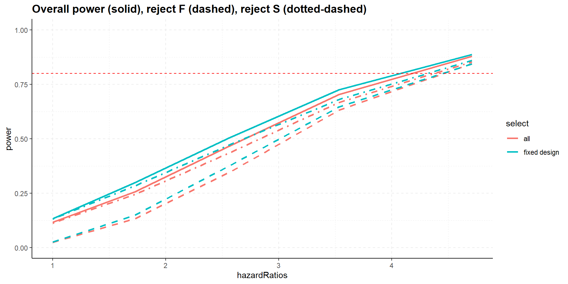
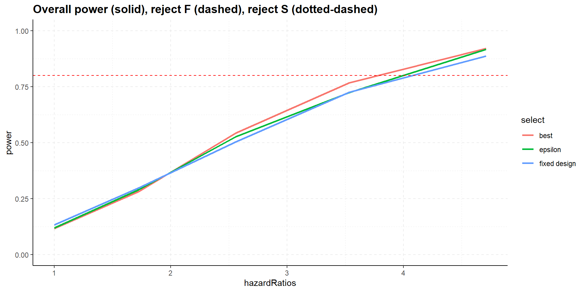
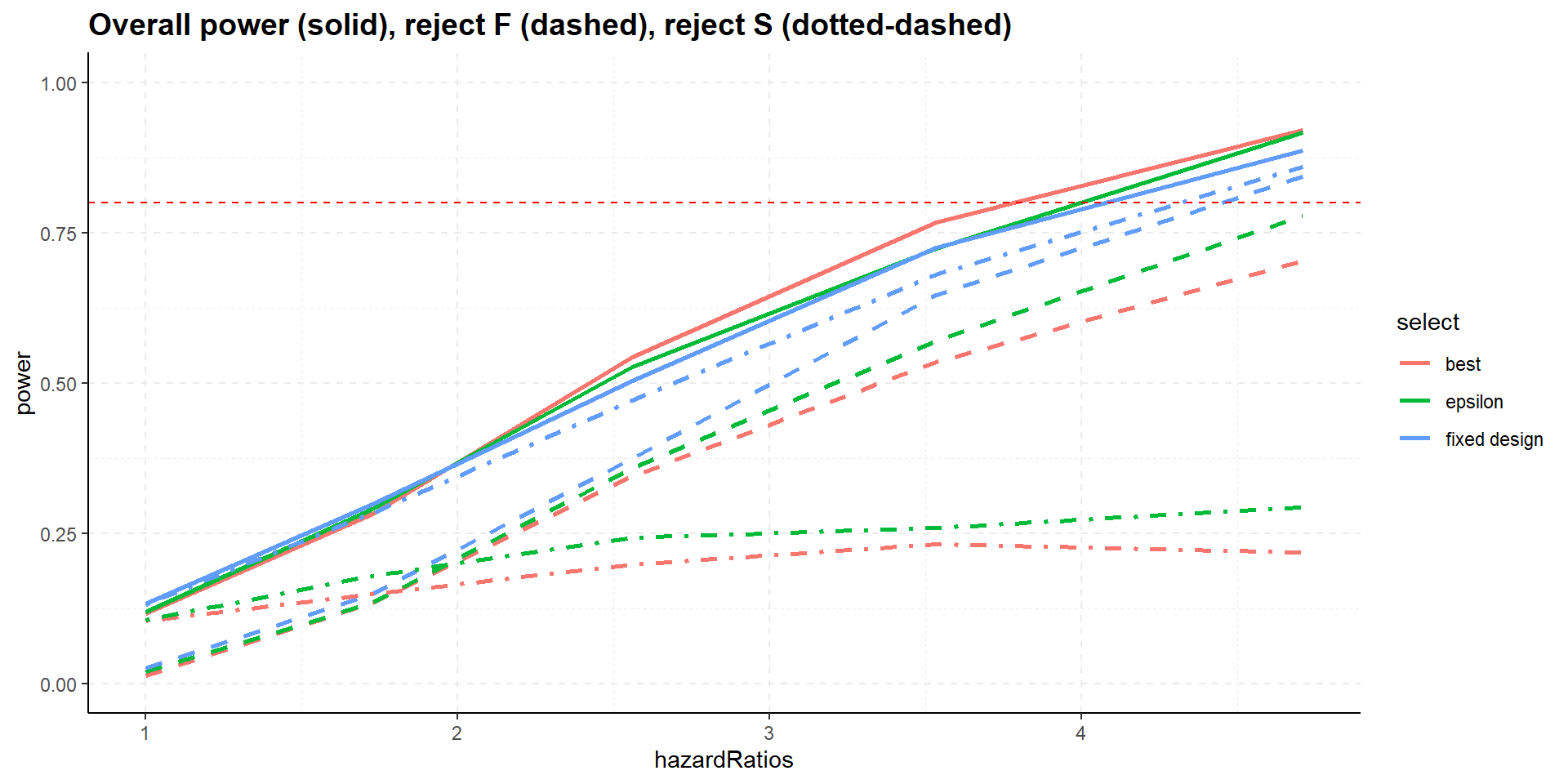
Summary
- All designs strongly control familywise error rate for testing \(H_0^F\) and \(H_0^S\).
- Selection increases overall power, i.e., showing significance in at least one population, S or F.
- Select the best, however, might decrease power for showing efficacy in F (and S), select the best inferior to epsilon rule.
- Rejecting both at stage 2 can be figured out, e.g., with
getData(simEnrichment3). - Other selection/enrichment rules and consideration of early efficacy might be interesting, too.
- Drop-outs cannot be taken into account since simulation for survival designs is not on the patient level (yet).
Questions?