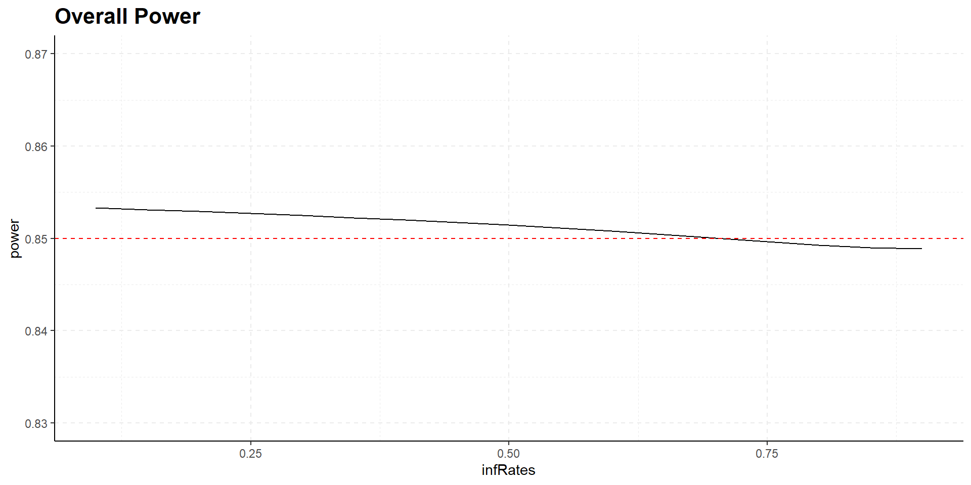
infRates <- seq(0.1, 0.9, 0.05)
power <- Vectorize(function(x) {
getDesignGroupSequential(
directionUpper = FALSE,
alpha = 0.025,
typeOfDesign = "asHSD",
gammaA = -4.5,
informationRates = c(x, 1)
) |>
getPowerSurvival(
hazardRatio = 0.563,
pi2 = 0.37,
eventTime = 6,
maxNumberOfEvents = 110,
maxNumberOfSubjects = 262,
accrualTime = 24
) |> fetch(overallReject)
})
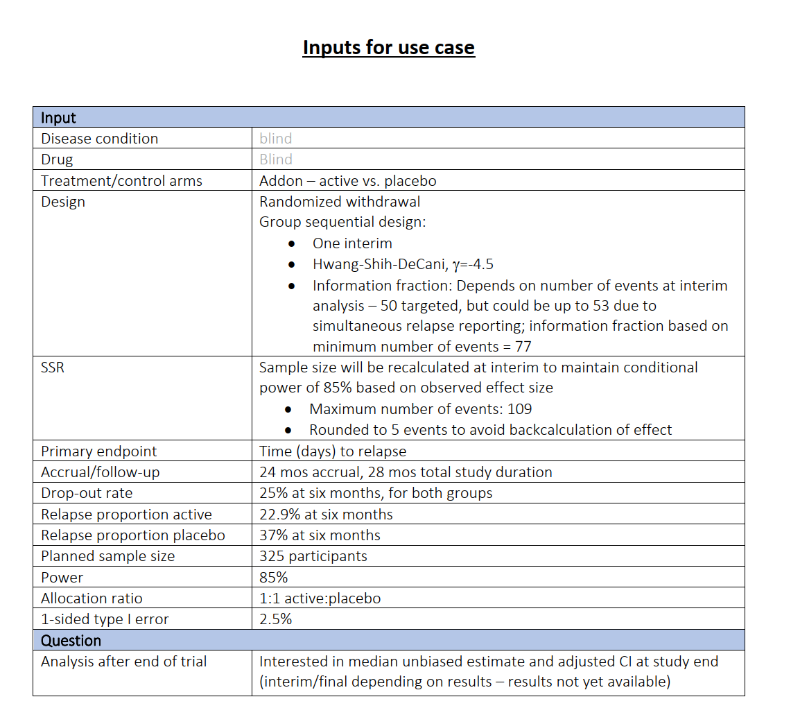
ggplot(data.frame(infRates = infRates, power = power(infRates)),
aes(infRates, power)
) +
geom_line() + ylim(0.83, 0.87) +
geom_hline(yintercept = 0.85, linetype = 2, lwd = 0.5, color = "red") +
ggtitle("Overall Power") +
theme_classic() + grids(linetype = "dashed") +
theme(plot.title=element_text(face='bold', size=16))Case Study Survival Design
Gernot Wassmer and Friedrich Pahlke
November 20, 2024
Case Study Survival Design
Survival Design
We wish to test
\(\hspace{2cm}H_0: \omega \geq 1 \text{ against } H_1: \omega < 1\)
We assume:
- \(\alpha = 0.025\)
- pi1 = 0.229, pi2 = 0.37 at 6 months
- Power \(1 - \beta = 0.85\) at \(\omega = \frac{\ln(1 - \text{pi1})}{\ln(1 - \text{pi2})} = 0.563\)
- Allocation ratio 1 : 1
rpact Planning
Start with fixed sample size (events) design:
library(rpact)
getSampleSizeSurvival(
  alpha = 0.025,
  beta = 0.15,
  hazardRatio = 0.563
) |> summary()
Sample size calculation for a survival endpoint
Fixed sample analysis, one-sided significance level 2.5%, power 85%. The results were calculated for a two-sample logrank test, H0: hazard ratio = 1, H1: hazard ratio = 0.563, control pi(2) = 0.2, event time = 12, accrual time = 12, accrual intensity = 57.4, follow-up time = 6.
| Stage | Fixed |
|---|---|
| Stage level (one-sided) | 0.0250 |
| Efficacy boundary (z-value scale) | 1.960 |
| Efficacy boundary (t) | 0.687 |
| Number of subjects | 689.1 |
| Number of events | 108.8 |
| Analysis time | 18.00 |
| Expected study duration under H1 | 18.00 |
Legend:
- (t): treatment effect scale
Required Number Of Events
109 events are needed to achieve 85% power for specified effect size
Required Number Of Subjects
Obviously, some default parameters were used to derive the required number of subjects
Design plan parameters and output for survival data
Design parameters
- Critical values: 1.960
- Significance level: 0.0250
- Type II error rate: 0.1500
- Test: one-sided
User defined parameters
- Hazard ratio: 0.563
Default parameters
- Theta H0: 1
- Type of computation: Schoenfeld
- Assumed control rate: 0.200
- Planned allocation ratio: 1
- Event time: 12
- Accrual time: 12.00
- kappa: 1
- Follow up time: 6.00
- Drop-out rate (1): 0.000
- Drop-out rate (2): 0.000
- Drop-out time: 12.00
Sample size and output
- Direction upper: FALSE
- Assumed treatment rate: 0.118
- median(1): 66.2
- median(2): 37.3
- lambda(1): 0.0105
- lambda(2): 0.0186
- Number of events: 108.8
- Accrual intensity: 57.4
- Number of events fixed: 108.8
- Number of subjects fixed: 689.1
- Number of subjects fixed (1): 344.6
- Number of subjects fixed (2): 344.6
- Analysis time: 18.00
- Study duration: 18.00
- Critical values (treatment effect scale): 0.687
Legend
- (i): values of treatment arm i
Study specifications
- accrual time = 24
- study duration = 28
- drop-out rate = 0.25 at 6 months
- planned number of participants = 325
Study specifications
Sample size calculation for a survival endpoint
Fixed sample analysis, one-sided significance level 2.5%, power 85%. The results were calculated for a two-sample logrank test, H0: hazard ratio = 1, H1: treatment pi(1) = 0.229, control pi(2) = 0.37, event time = 6, accrual time = 24, accrual intensity = 10.8, follow-up time = 4, dropout rate(1) = 0.25, dropout rate(2) = 0.25, dropout time = 6.
| Stage | Fixed |
|---|---|
| Stage level (one-sided) | 0.0250 |
| Efficacy boundary (z-value scale) | 1.960 |
| Efficacy boundary (t) | 0.687 |
| Number of subjects | 259.2 |
| Number of events | 108.7 |
| Analysis time | 28.00 |
| Expected study duration under H1 | 28.00 |
Legend:
- (t): treatment effect scale
Follow-up time can be reduced with 325 participants:
getSampleSizeSurvival(
    alpha = 0.025,
    beta = 0.15,
    pi1 = 0.229,
    pi2 = 0.37,
    eventTime = 6,
    accrualTime = 24,
    maxNumberOfSubjects = 325,
    dropoutRate1 = 0.25,
    dropoutRate2 = 0.25,
    dropoutTime = 6
) |> summary()
Sample size calculation for a survival endpoint
Fixed sample analysis, one-sided significance level 2.5%, power 85%. The results were calculated for a two-sample logrank test, H0: hazard ratio = 1, H1: treatment pi(1) = 0.229, control pi(2) = 0.37, number of subjects = 325, event time = 6, accrual time = 24, accrual intensity = 13.5, dropout rate(1) = 0.25, dropout rate(2) = 0.25, dropout time = 6.
| Stage | Fixed |
|---|---|
| Stage level (one-sided) | 0.0250 |
| Efficacy boundary (z-value scale) | 1.960 |
| Efficacy boundary (t) | 0.687 |
| Number of subjects | 325.0 |
| Number of events | 108.7 |
| Analysis time | 23.18 |
| Expected study duration under H1 | 23.18 |
Legend:
- (t): treatment effect scale
Design with interim stage
designGS <- getDesignGroupSequential(
    directionUpper = FALSE,
    alpha = 0.025,
    beta = 0.15,
    typeOfDesign = "asHSD",
    gammaA = -4.5,
    informationRates = c(50/77, 1)
)
getSampleSizeSurvival(
    design = designGS,
    pi1 = 0.229,
    pi2 = 0.37,
    eventTime = 6,
    accrualTime = 24,
    followUpTime = 4,
    dropoutRate1 = 0.25,
    dropoutRate2 = 0.25,
    dropoutTime = 6
) |> summary()
Design with interim stage
Sample size calculation for a survival endpoint
Sequential analysis with a maximum of 2 looks (group sequential design), one-sided overall significance level 2.5%, power 85%. The results were calculated for a two-sample logrank test, H0: hazard ratio = 1, H1: treatment pi(1) = 0.229, control pi(2) = 0.37, event time = 6, accrual time = 24, accrual intensity = 10.9, follow-up time = 4, dropout rate(1) = 0.25, dropout rate(2) = 0.25, dropout time = 6.
| Stage | 1 | 2 |
|---|---|---|
| Planned information rate | 64.9% | 100% |
| Cumulative alpha spent | 0.0049 | 0.0250 |
| Stage levels (one-sided) | 0.0049 | 0.0235 |
| Efficacy boundary (z-value scale) | 2.580 | 1.985 |
| Efficacy boundary (t) | 0.543 | 0.685 |
| Cumulative power | 0.4388 | 0.8500 |
| Number of subjects | 219.7 | 261.7 |
| Expected number of subjects under H1 | 243.3 | |
| Cumulative number of events | 71.3 | 109.8 |
| Expected number of events under H1 | 92.9 | |
| Analysis time | 20.15 | 28.00 |
| Expected study duration under H1 | 24.56 | |
| Exit probability for efficacy (under H0) | 0.0049 | |
| Exit probability for efficacy (under H1) | 0.4388 |
Legend:
- (t): treatment effect scale
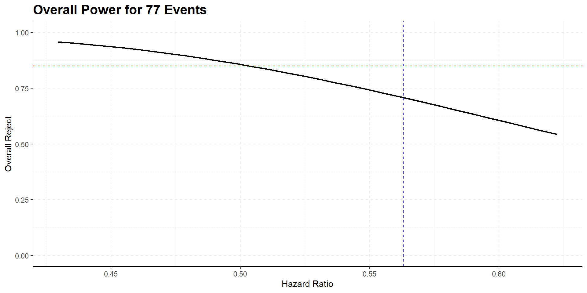
Results
110 events are needed to achieve 85% power
262 study participants are needed to expect required number of events at given accrual and follow-up
drop-outs taken into account
325 planned participants are expected to achieve study goal in a shorter time frame
77 events do not achieve power 85%
Overall Power for 77 events
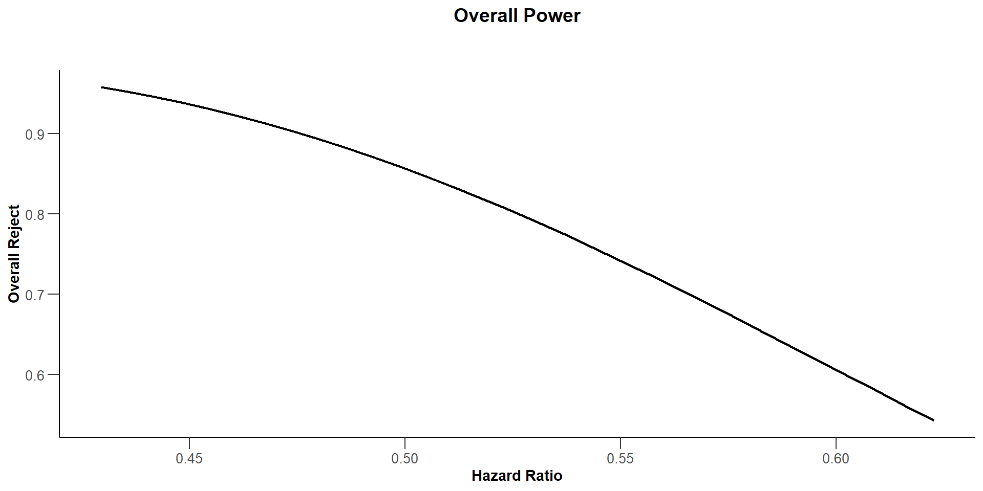
library(ggplot2)
library(ggpubr) # This for the grids
getPowerSurvival(
    design = designGS,
    pi1 = c(0.18, 0.25),
    pi2 = 0.37,
    eventTime = 6,
    maxNumberOfEvents = 77,
    maxNumberOfSubjects = 262,
    accrualTime = 24,
    dropoutRate1 = 0.25,
    dropoutRate2 = 0.25,
    dropoutTime = 6
) |> plot(type = 7) +
ylim(0, 1) +
ggtitle("Overall Power for 77 Events") +
geom_vline(xintercept = 0.563, linetype = 2, lwd = 0.5, color = "blue") +
geom_hline(yintercept = 0.85, linetype = 2, lwd = 0.5, color = "red") +
theme_classic() + grids(linetype = "dashed") +
theme(plot.title=element_text(face = 'bold', size = 16)
) 
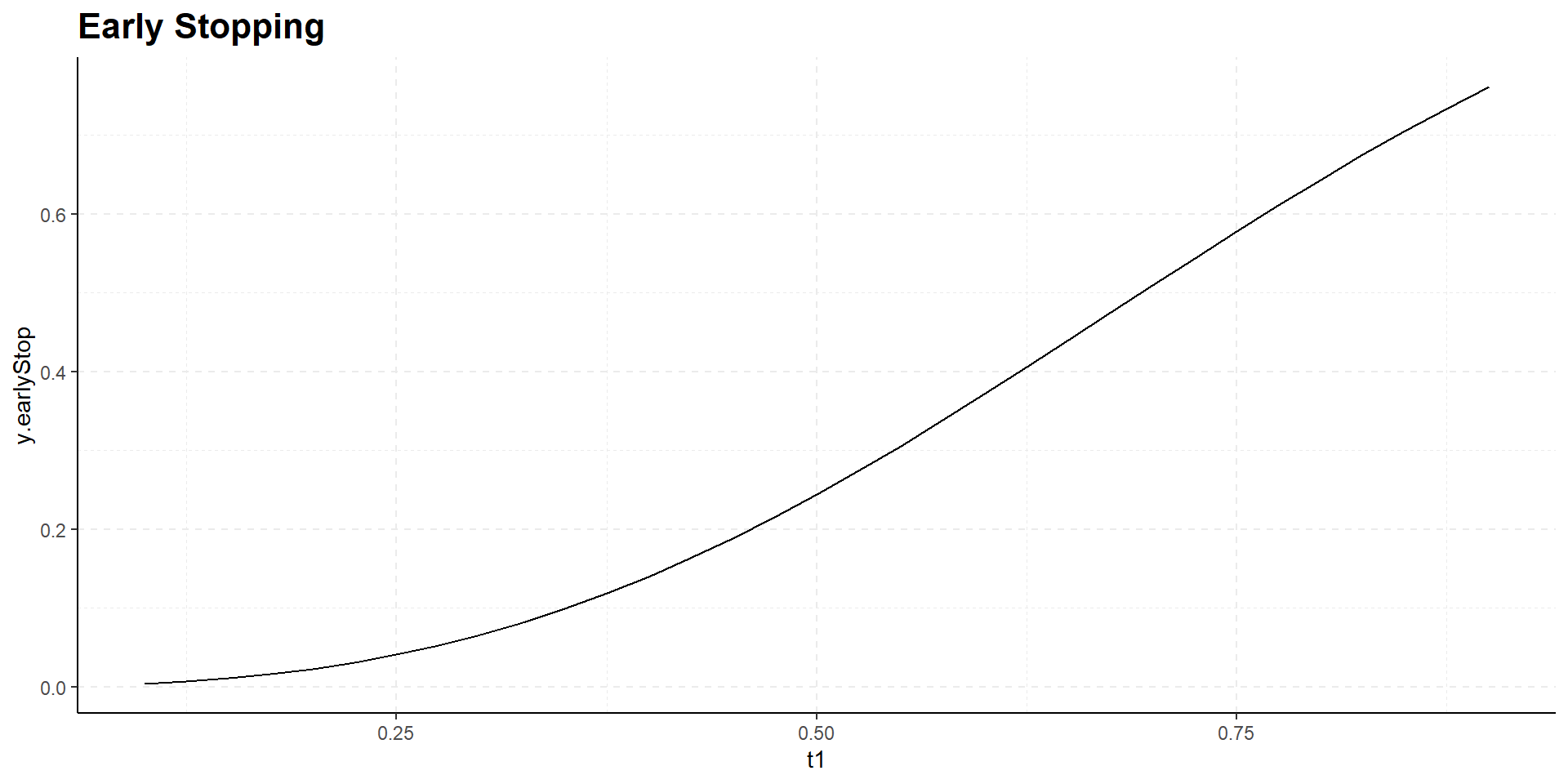
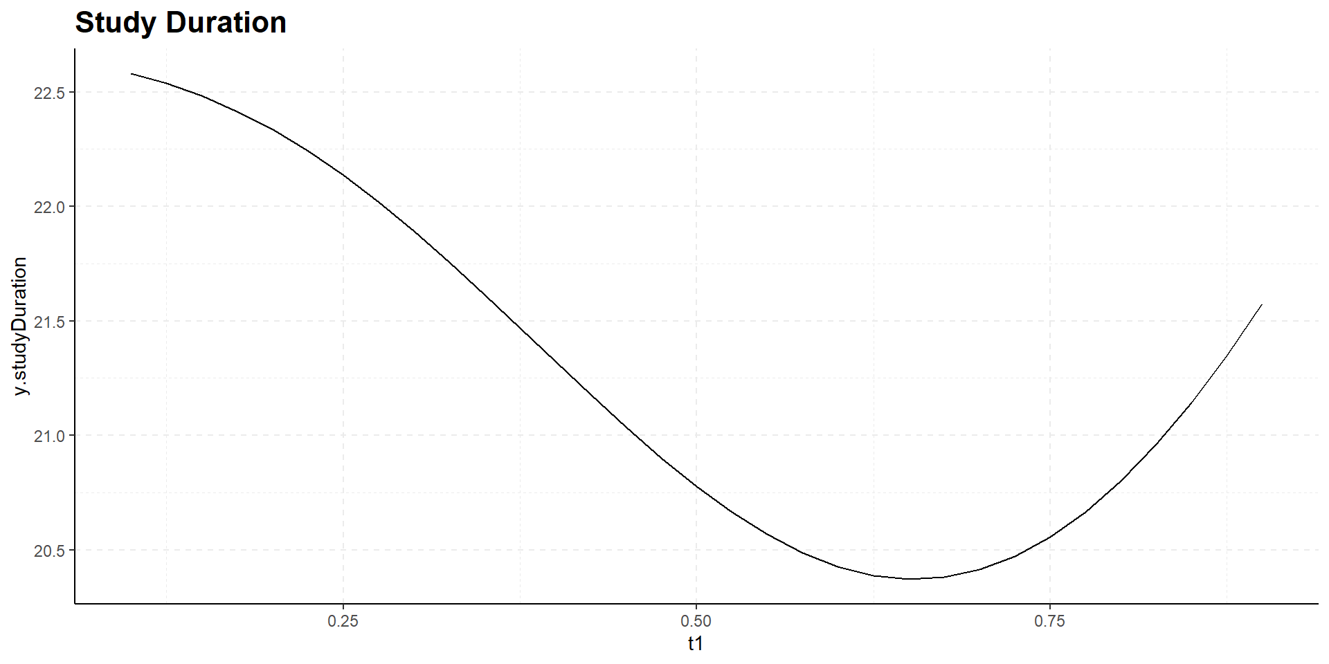
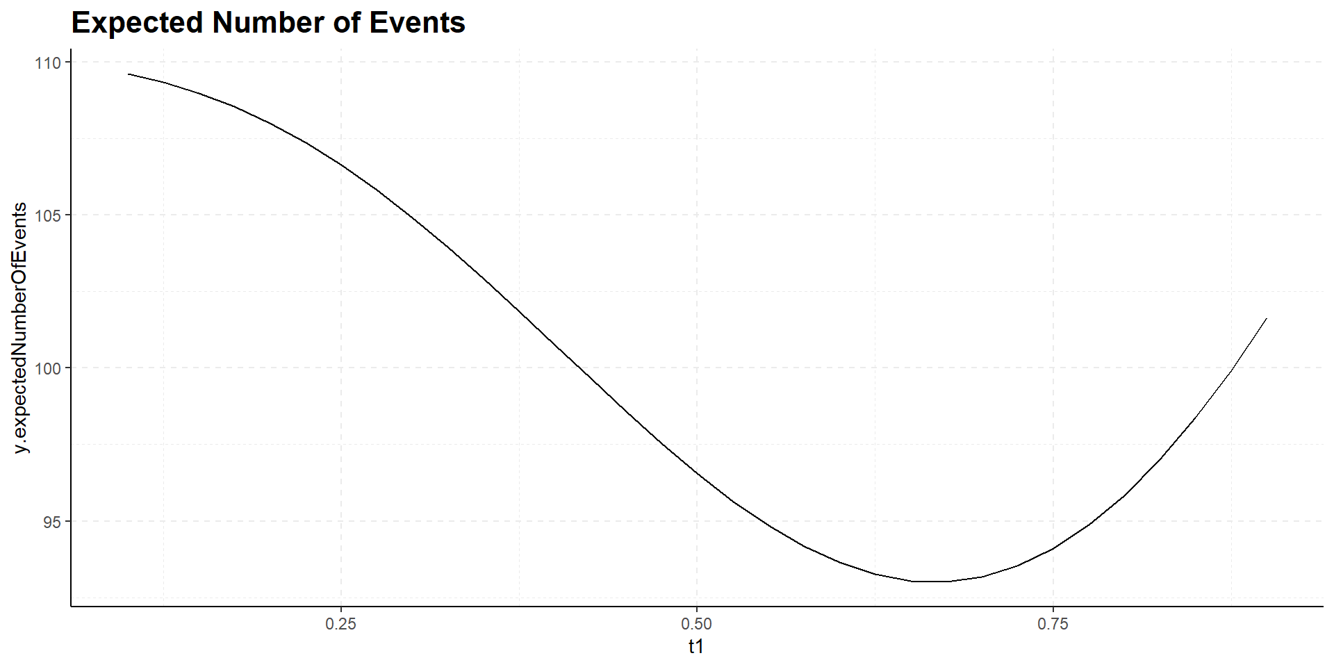
When should the interim take place?
Varying interim time has no relevant influence on power
When should the interim take place?
Interim time point has negligible influence on power but has effect on expected study duration, i.e., on expected number of events:
Design Considerations
- Perform interim after observation of 77 events, then consider event number recalculation (“SSR”)
- Use combination testing principle with pre-fixed weight for flexible recalculation.
- Constrained promizing zone approach as a useful strategy.
For use in rpact, see Vignette Promizing Zone Design with rpact. - Analysis of trial according to Vignette Analysis of a Group Sequential Trial with a Survival Endpoint using rpact.
- Conditional power calculation, calculation of repeated and final confidence intervals and p-values provided therein.
Questions?